TetraProbe Specs and Performance Tests

TetraLite Products
TetraProbe
An Low-cost Digitizing Probe for CNC Applications.
Home | Description | Performance | Order | Contact

Test Results

A Repeatability Test in Which I Reveal That My Mill Is Not Perfect and Neither Is My Probe But Both Are Better Than I Might Have Imagined

This test used G-code generated by the digitizing wizard (not the digitizing plug-in) in Artsoft Controls Mach3 Version R2.0.065. The wizard was set up to scan an area 1.0" wide (X) by 0.5" high (Y) with X and Y steps of 0.025" resulting in a 40 by 20 point sampling grid with a total of 800 sample point. The object scanned is an area on the table on my Taig mill. The table on my mill is like new, the way it came from the factory and is undamaged in case you are wondering. The G-code was run six times in a row, saving the outputted point cloud files each time. These 6 point cloud files were then processed using the Global Mapper program by first importing them with a scale factor on all three (X, Y and Z) axes of 100,000. This was done because Global Mapper does not work in inches, but defaults to meters as its basic unit of measurement. By scaling up a factor of 100,000, the least significant digit from the point cloud files (the 100-thousandths place) becomes the unit meters digit (the digit in the "ones" place in the resulting units). For example, a Z axis reading of -0.02019 is converted to -2019 meters -- an absolute unit scaling factor of 100,000. The resulting elevations in Global Mapper are then offset in order to make them positive numbers with the lowest elevation brought up to zero. This is easily done because Global Mapper tells you the lowest and highest elevations in the file, so all I did was add the absolute value of the lowest point to all points by adding the offset, bringing them all up so that the lowest point is at zero. At this point in Global Mapper, the resulting elevations are now positive values within the range from lowest to highest. If the probe were perfect, that number would indicate the greatest difference in elevation points on the mill table. If the probe and the table were perfect all points would be normalized to zero.

The images below were generated in Global Mapper and contour lines were overlayed (also in Global Mapper) at 0.5 meter (5 millionths of an inch) intervals. Relative locations in these images that look similar indicate more nearly the actual error of the mill table. Relative locations that look different indicate errors of the probe. Both errors can readily be seen in the images below.

The colors range from lowest to highest in the order: blue, green, yellow, orange, red with transition colors in between. This shading method is known as "atlas shading".

It can be inferred from these scans that the section of my mill table scanned in these tests is obviously higher at lower values of Y, or, in other words, it slopes down toward the back of the machine with an difference in height in the 0.5" Y travel that was scanned of something less than 0.00016" and perhaps roughly half that amount.

It can be further inferred from these scans that the Z axis measurement error of the probe cannot be more than 0.00022" (the greatest difference in elevations of all six scans) and is obviously less than that because of the slope of the mill table and anomalies on the surface of the table. You can see small high and low spots and areas that are in the same location on all six images. These indicate "faults" of the table (or real vertical anomalies of the surface). You can also see relative locations that are at different elevations from one image to the other. These indicate probe errors (and to a lesser extent I suppose, Z axis anomalies of the mill).

Ambient temperature changes during these test occured but were not documented. Their effect is presumed to be extremely small in these results.

To get a better look at these images and a clearer view of the contour lines, download the image and zoom in on it in your image viewer.

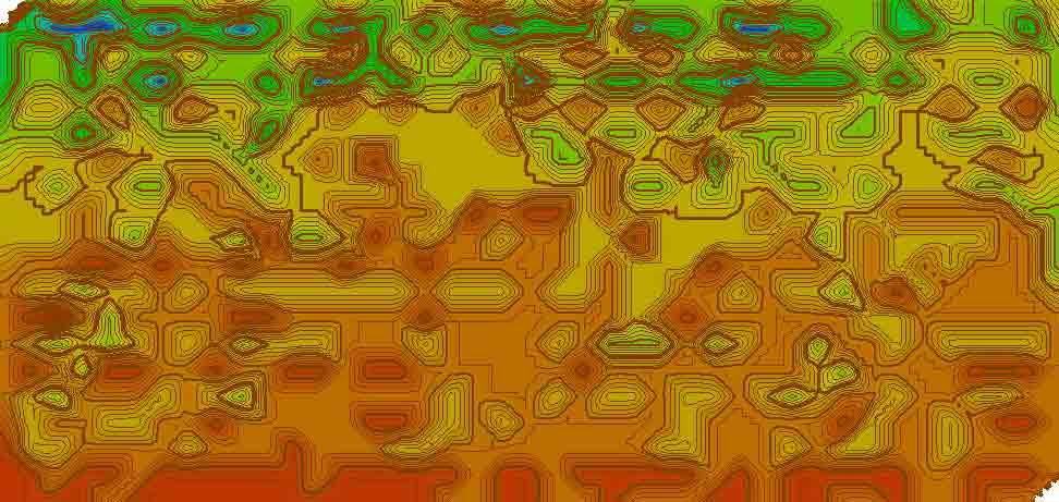	Scan 1 MIN ELEVATION = -2016 meters (-0.02016") MAX ELEVATION = -1997 meters (-0.01997") Difference = 19 meters (0.00019")
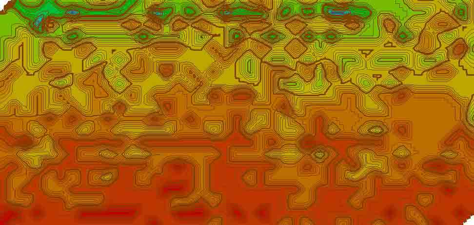	Scan 2 MIN ELEVATION = -2016 meters (-0.02016") MAX ELEVATION = -1997 meters (-0.01997") Difference = 19 meters (0.00019")
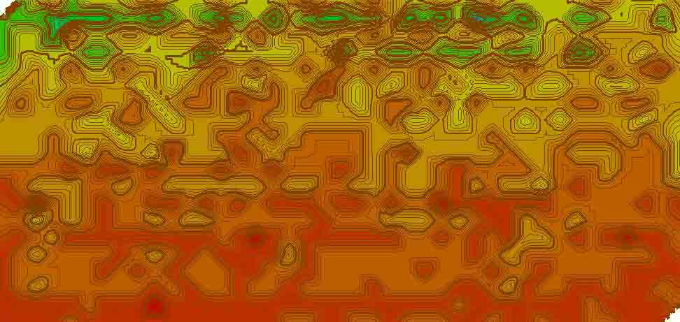	Scan 3 MIN ELEVATION = -2019 meters (-0.02019") MAX ELEVATION = -1997 meters (-0.01997") Difference = 22 meters (0.00022")
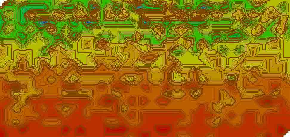	Scan 4 MIN ELEVATION = -2019 meters (-0.02019") MAX ELEVATION = -1997 meters (-0.01997") Difference = 22 meters (0.00022")
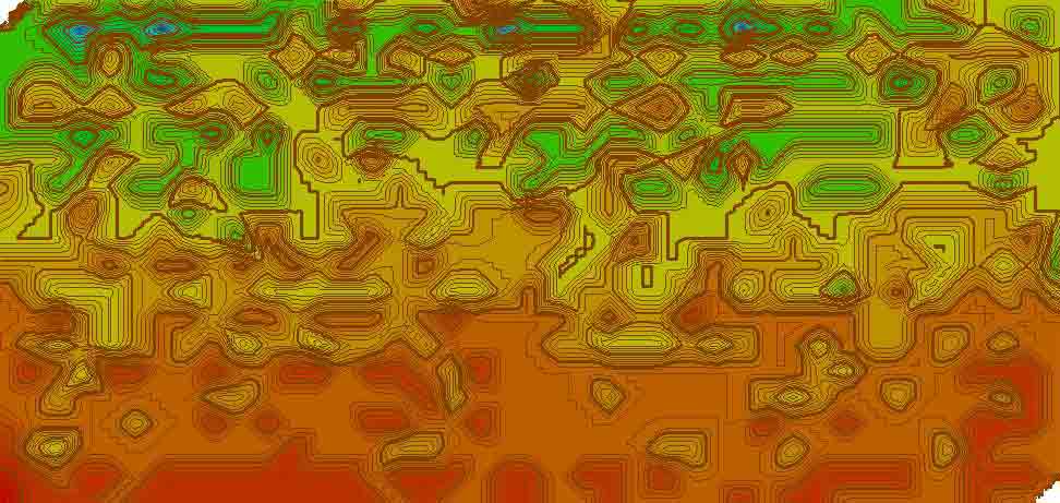	Scan 5 MIN ELEVATION = -2019 meters (-0.02019") MAX ELEVATION = -1997 meters (-0.01997") Difference = 22 meters (0.00022")
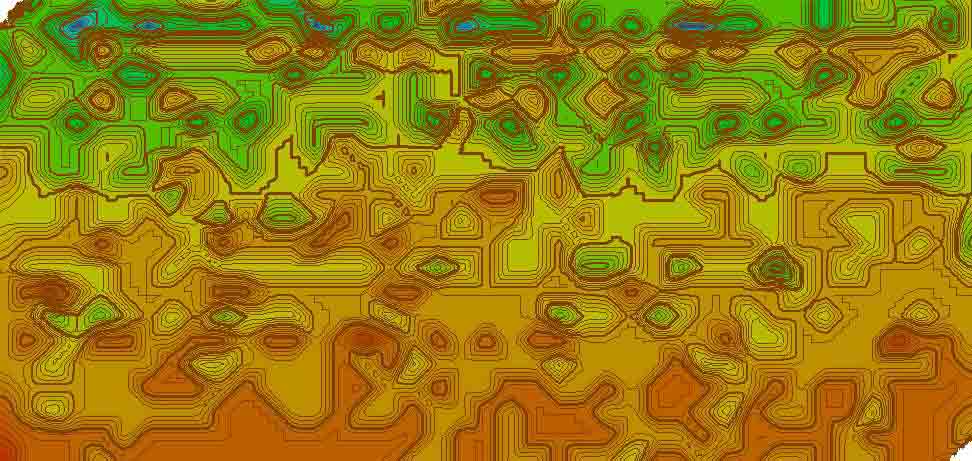	Scan 6 MIN ELEVATION = -2016 meters (-0.02016") MAX ELEVATION = -1997 meters (-0.01997") Difference = 19 meters (0.00019")

Looking at these images it can be seen that many high and low spots are detected in the same locations indicating actual variations of the mill table surface. Although it looks rather rough overall, keep in mind that the maximum variation we are seeing on all these scans is 0.00022" or less.

The contour lines are 5 millionths of an inch (0.000005" or 0.127 microns) apart in elevation. Yikes! that's about 1/8th of a micron! But remember that these contours lines represent extrapolated elevations in between the actual measurement points, so the probe and the milling machine are in no way capable of resolution this fine.